Consider a complex column vector \begin{equation} v = \begin{pmatrix}b\cr c\cr\end{pmatrix} \label{column} \end{equation} where $b,c\in\CC$. What can we do with $v$? Well, we can take its Hermitian conjugate, defined as before, namely \begin{equation} v^\dagger = \begin{pmatrix}\bar{b}& \bar{c}\cr\end{pmatrix} \end{equation} We can now multiply $v$ and $v^\dagger$ in two quite different ways. We can produce a complex number \begin{equation} v^\dagger v = |b|^2 + |c|^2 \label{scalar} \end{equation} and, if we multiply in the opposite order, a matrix \begin{equation} v v^\dagger = \begin{pmatrix} |b|^2& b\bar{c}\cr \noalign{\smallskip} c\bar{b}& |c|^2 \end{pmatrix} \end{equation}

One way to visualize $v$ is to think of it as a point in $\CC^2=\RR^4$, in which case (\ref{scalar}) is just the usual (squared) vector norm. Suppose we normalize $v$ by requiring that $v^\dagger v = 1$. Then $v$ lies on the unit sphere in $\RR^4$, which is 3-dimensional, and hence denoted by $\SS^3$.

What about $vv^\dagger$? This matrix is Hermitian! As discussed in § 9.3, We can therefore identify $vv^\dagger$ with a vector in spacetime, via \begin{align} t+z &= |b|^2 \\ t-z &= |c|^2 \\ x+iy &= c\bar{b} \end{align} We can invert these relationships, obtaining 1) \begin{align} t &= \frac12\, (|b|^2 + |c|^2) \\ z &= \frac12\, (|b|^2 - |c|^2) \\ x &= \frac12\, (c\bar{b} + b\bar{c}) \\ iy &= \frac12\, (c\bar{b} - b\bar{c}) \end{align} The normalization (\ref{scalar}) of $v$ tells us that $t$ is constant, which also follows immediately from \begin{equation} 2t = \tr(vv^\dagger) = v^\dagger v = 1 \end{equation} So the trace of $vv^\dagger$ is special; what about its determinant? We have \begin{equation} \det(vv^\dagger) = |b|^2 |c|^2 - (b\bar{c})(c\bar{b}) = |b|^2 |c|^2 - |b\bar{c}|^2 = |b|^2 |c|^2 - |bc|^2 = 0 \label{division} \end{equation} Thus, $vv^\dagger$ represents a null vector! Putting this all together, we have \begin{equation} x^2 + y^2 + z^2 = t^2 = \hbox{constant} \end{equation} so that we can think of $vv^\dagger$ as a point on a particular sphere, which we denote $\SS^2$.

We have constructed a famous map between $\SS^3$ and $\SS^2$ known as the Hopf map, and which for us is simply given by \begin{align} \SS^3 &\longrightarrow  \SS^2 \nonumber\\ v  &\longmapsto vv^\dagger \label{Hopf} \end{align} This map is not one-to-one. After all, it takes 3 angles to specify a point in $\SS^3$, but only 2 to specify a point in $\SS^2$.

What information have we lost in “squaring” $v$ to get $vv^\dagger$? If we multiply $v$ by a phase, that is, a complex number of the form $e^{i\theta}$, then not only is the norm (\ref{scalar}) unchanged, but also the square! Explicitly, if \begin{equation} w = v e^{i\theta} \label{phase} \end{equation} then \begin{equation} ww^\dagger = vv^\dagger \label{square} \end{equation} This phase freedom is associated with the circle $\SS^1$ of unit complex numbers — which includes antipodal points as a special case. This copy of $\SS^1$ is in fact also a group, denoted $U(1)$, since the product of any two unit complex numbers is another such number.

Not surprisingly, the above construction works over any of the division algebras. Note the crucial use of the division algebra property in (\ref{division}) to conclude that $vv^\dagger$ is a null vector! Thus, allowing the components of $v$ in turn to be in $\RR$, $\CC$, $\HH$, and $\OO$ results in $vv^\dagger$ being a null vector in 3, 4, 6, or 10 spacetime dimensions, respectively. Imposing the normalization condition (\ref{scalar}) allows $vv^\dagger$ to be thought of as a point on the spheres $\SS^1$, $\SS^2$, $\SS^4$, and $\SS^8$, respectively, while $v$ can be interpreted as a point on the spheres $\SS^1$, $\SS^3$, $\SS^7$, and $\SS^{15}$, respectively.

There are a couple of details to check. Over $\HH$, it is essential that the phase freedom in (\ref{phase}) be written on the right. And of course the phase is given by an arbitrary unit quaternion, corresponding to $\SS^3$. Over $\OO$, we must be even more careful in identifying the phase freedom; there appear to be associativity issues in the transition from (\ref{phase}) to (\ref{square}). However, there is a way around this: $vv^\dagger$ is really complex, since it contains only one octonionic direction. It therefore admits a complex “square root” $u$. If we apply the phase freedom to $u$, rather than $v$, the computation becomes quaternionic; the associativity problems disappear. Explicitly, choosing 2) \begin{equation} u = \begin{pmatrix} {b\bar{c}\over|c|}\cr \noalign{\smallskip} |c|\cr \end{pmatrix} \label{octohopf} \end{equation} we have \begin{equation} uu^\dagger = vv^\dagger \end{equation} and the most general column vector $w$ satisfying (\ref{square}) is \begin{equation} w = u\xi \end{equation} where the phase $\xi$ is any unit octonion, which can be thought of as an element of $\SS^7$. We can recover $v$ by putting $\xi={c\over|c|}$.

Putting this all together, we obtain the four Hopf maps \begin{align} \SS^{15} &\longrightarrow  \SS^8 \nonumber\\ \SS^7  &\longrightarrow  \SS^4 \nonumber\\ \SS^3  &\longrightarrow  \SS^2 \\ \SS^1  &\longrightarrow  \SS^1 \nonumber \end{align} It is remarkable that there are precisely four of these maps. It is even more remarkable that they are related to the four division algebras.

 
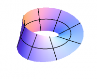
Figure 1: A Möbius strip.

What do the Hopf maps look like? Consider first a Möbius strip, as shown in Figure 1. The Möbius strip is an example of a fiber bundle, in which there is a base manifold, in this case the circle in the center of the Möbius strip, and a fiber, in this case a line segment, otherwise known as the 1-dimensional disk, $D^1$. The Möbius strip is therefore a fiber bundle over $\SS^1$, with fiber $D^1$. This bundle is nontrivial; it is not simply $\SS^1\times D^1$, which would be a cylinder.

 
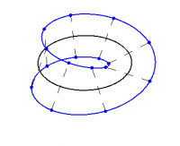
Figure 2: The smallest Hopf bundle.

If we now change the fibers by removing all but the endpoints of each line segment, we are left with the fiber bundle shown in Figure 2. The base space is still $\SS^1$, but the fibers now consist of two points, which is the 0-sphere, $S^0$, consisting of all points in the line that lie a unit distance from the origin. But these points also make up a circle! Thus, this fiber bundle is itself $\SS^1$, over $\SS^1$, with fiber $S^0$ — precisely the smallest fiber bundle as given above.

 
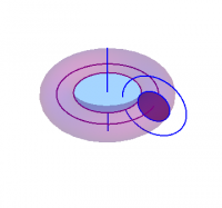
Figure 3: The Hopf bundle.

What about the next case, of $\SS^3$ over $\SS^2$, which is the original Hopf map? The Hopf map is also referred to as the Hopf bundle, because it describes $\SS^3$ as a fiber bundle with base space $\SS^2$ and fiber $\SS^1$; roughly speaking, there is a copy of $\SS^1$, given by the phase freedom, at each point of $\SS^2$. For the Möbius strip, we obtained the fibre $\SS^0$ as the boundary of $D^1$; we apply the same idea here. Since $\SS^3$ is the boundary of $D^4$, the disk (“ball”) in 4 dimensions, we have \begin{align} \SS^3 &= \partial D^4 = \partial (D^2\times D^2) \nonumber\\ &= (\partial D^2\times D^2) \cup (D^2\times\partial D^2) \nonumber\\ & = (\SS^1\times D^2) \cup (D^2\times\SS^1) \nonumber\\ &\cong \RR^3 \cup \{\infty\} \end{align} Thus, we can represent $\SS^3$ as the points in $\RR^3$, together with a point at infinity, as shown in Figure 3. There are two disks ($D^2$) shown in this figure, one inside the torus, the other in the $xy$ plane, in the middle of the torus, but outside it. Each disk represents a hemisphere of the basespace, with the circles that intersect the disks representing the fibres. 3)

The geometric representations of the first two Hopf bundles shown in Figures 2 and 3. is purely topological, as it fails to show the normalization used in our algebraic construction above.